Greatest common divisor and Euclidean algorithm

Subsection 5.3.3 Greatest common divisor and Euclidean algorithm

Definition 5.3.3.1.

Let \(a\) and \(b\) be integers, not both \(0\text{.}\) The greatest common divisor of \(a\) and \(b\text{,}\) denoted \(\gcd(a,b)\text{,}\) is the largest integer \(d\) such that \(d \mid a\) and \(d \mid b\text{.}\) We say \(a\) is relatively prime or coprime to \(b\) if \(\gcd(a,b) = 1\text{.}\)

🔗

Remark 5.3.3.2.

It is easy to see from the definition that \(\gcd(a,b) = \gcd(b,a)\text{.}\)

🔗

Example 5.3.3.3. Greatest common divisor.

The greatest common divisor of \(10\) and \(15\) is \(5\) since \(5\) divides both \(10\) and \(15\text{,}\) and it is the largest integer to do so. We write \(\gcd(10,15) = 5\text{.}\)

🔗

The integers \(15\) and \(22\) are relatively prime since \(\gcd(22,15) = 1\text{.}\)

🔗

Example 5.3.3.4. Special cases of greatest common divisors.

Let \(a\in\NN\) and \(b\in\NN\text{.}\) Then

\(\gcd(a,b)=\gcd(b,a)\text{,}\)
🔗

🔗
\(\gcd(a,a)=a\text{,}\) as the largest natural number that divides \(a\) is \(a\text{.}\)
🔗

🔗
\(\gcd(a,0)=a\text{,}\) as \(0\) is divisible by all natural numbers \(a\text{.}\)
🔗

🔗
\(\gcd(a,1)=1\text{,}\) as the largest divisor of \(1\) is \(1\) and all natural numbers \(a\) are divisible by \(1\text{.}\)
🔗

🔗

🔗

Definition 5.3.3.5.

For a positive integer \(n\text{,}\) the Euler phi function or Euler totient function evaluated at \(n\text{,}\) denoted \(\phi(n)\text{,}\) is the number of non-negative integers less than \(n\) that are relatively prime to \(n\text{.}\)

🔗

Example 5.3.3.6. Relatively prime to \(10\).

There are four positive integers less than \(10\) that are relatively prime to \(10\text{:}\) \(\set{1, 3, 7, 9}\text{.}\) Thus \(\phi(10) = 4\text{.}\)

🔗

Example 5.3.3.7. Relatively prime to \(7\).

There are six positive integers less than \(7\) that are relatively prime to \(7\text{:}\) \(\set{1,2, 3,4,5,6}\text{.}\) Thus \(\phi(7) = 6\text{.}\)

🔗

Remark 5.3.3.8.

For \(p\) prime, it is easy to show that \(\phi(p) = p-1\text{.}\) One can also show that for \(p\) and \(q\) distinct primes, \(\phi(pq) = (p-1)(q-1)\text{.}\)

🔗

Definition 5.3.3.9.

Let \(a\) and \(b\) be positive integers. The least common multiple of \(a\) and \(b\text{,}\) denoted \(\lcm(a,b)\text{,}\) is the smallest positive integer \(\ell\) such that \(a \mid \ell\) and \(b \mid \ell\text{.}\)

🔗

For integers we can factor, or for small integers where we can use trial division, it is straightforward to compute greatest common divisors and least common multiples.

🔗

Example 5.3.3.10. Greatest common divisor and least common multiple.

Let’s compute the greatest common divisor and least common multiple of \(24\) and \(30\text{.}\) We have that \(24 = 2^3 \cdot 3\text{,}\) and \(30 = 2 \cdot 3 \cdot 5\text{.}\) They have \(2 \cdot 3\) in common, so greatest common divisor is

\begin{equation*} \gcd(30, 24) = 2 \cdot 3 = 6. \end{equation*}

For the least common multiple, we need to include all the prime factors that arise and keep the larger exponent, so the least common multiple is

\begin{equation*} \lcm(30, 24) = 2^3 \cdot 3 \cdot 5 = 120. \end{equation*}

Note that \(24 \cdot 30 = 720 = 6 \cdot 120\) so that

\begin{equation*} 24 \cdot 30 = \gcd(30, 24)\lcm(30, 24). \end{equation*}

This turns out to be true in general. See Theorem 5.3.3.11.

🔗

Theorem 5.3.3.11.

Let \(a\) and \(b\) be positive integers. Then

\begin{equation*} ab = \gcd(a,b)\lcm(a,b) \end{equation*}

🔗

Proof.

Try this at home. Hint: Use the prime factorizations of \(a\) and \(b\) guaranteed from the Fundamental Theorem of Arithmetic. Express the gcd and lcm of \(a\) and \(b\) in terms of the factorizations. Compare the product of these with the prime factorization of the product of \(a\) and \(b\text{.}\)

🔗

Factoring or trial division works for computing greatest common divisors, but for large \(a\) and \(b\text{,}\) it is horribly inefficient. There is a better method known as the Euclidean algorithm . As an additional bonus, the theorem above shows that fast computation of gcd leads to fast computation of lcm. The Euclidean algorithm works because of the following results.

🔗

Theorem 5.3.3.12.

Let \(g\) be a natural number and let \(a\text{,}\) \(b\text{,}\) and \(q\) be integers.

If \(g\) divides \(a\) and \(g\) divides \(b\) then \(g\) also divides \(a-(b\cdot q)\text{.}\)
🔗

🔗
If \(g\) divides \(a-(b\cdot q)\) and \(g\) divides \(b\) then \(g\) also divides \(a\text{.}\)
🔗

🔗

🔗

Proof.

As \(g\) divides \(a\) there exists an integer \(s\) such that \(a=g\cdot s\text{.}\)\\ As \(g\) divides \(b\) there exists an integer \(t\) such that \(b=g\cdot t\text{.}\)\\ We now have

\begin{equation*} a-(b\cdot q)=(g\cdot s)-((g\cdot t) \cdot q)=g\cdot(s-(t\cdot q)). \end{equation*}

Thus \(a-(b\cdot q)\) is a multiple of \(g\) which means that \(g\) divides \(a-(b\cdot q)\text{.}\)

🔗

🔗
As \(g\) divides \(a-(b\cdot q)\) there exists an integer \(s\) such that \(a-(b\cdot q)=g\cdot s\text{.}\)
🔗

As \(g\) divides \(b\text{,}\) there exists an integer \(s\) such that \(b=g\cdot t\text{.}\)
🔗

We now have

\begin{equation*} a=(a-(b\cdot q))+ (b\cdot q)= (g\cdot s)+( (g\cdot t)\cdot q)=g\cdot(s+(t\cdot q)) \end{equation*}

Thus \(a\) is a multiple of \(g\) which means that \(g\) divides \(a\text{.}\)

🔗

🔗

🔗

Theorem 5.3.3.13.

Let \(g\) be a natural number and let \(a\text{,}\) \(b\text{,}\) and \(q\) be integers.

\(\displaystyle \gcd(a-(b\cdot q),b)=\gcd(a,b)\)
🔗

🔗
\(\gcd(a\bmod b,b)=\gcd(a,b)\text{.}\)
🔗

🔗

🔗

Proof.

By the theorem above natural numbers \(g\) that divide \(a\) and \(b\) also divide \(a-(b\cdot q)\text{.}\)
🔗

All natural numbers \(g\) that divide \(a-(b\cdot q)\) and \(b\) also divide \(a\text{.}\)
🔗

Thus the common divisors of \(a\) and \(b\) and the common divisors of \(a-(b\cdot q)\) are the same.
🔗

So, in particular, the greatest common divisor of \(a\) and \(b\) is equal to the greatest common divisor of \(a-(b\cdot q)\) and \(b\text{.}\)
🔗

🔗
For \(q=a \div q\) we have \(a \bmod b=a-(b\cdot q)\text{.}\)
🔗

We get

\begin{equation*} \gcd(a\bmod b,b) = \gcd(a-(b\cdot q),b) = \gcd(a,b) \end{equation*}

🔗

🔗

🔗

It may look like these Theorems do not help, as it just turns one gcd computation into another. The real power here comes from two facts:

\(\gcd(a,b) = \gcd(b,a)\text{,}\) so we can arrange that \(b\) is
🔗

🔗
\(a \bmod b\) is strictly less than \(b\text{.}\)
🔗

🔗

That means that Theorem 5.3.3.13 allows us to compute \(\gcd(a, b)\) by computing \(\gcd(A,B)\text{,}\) where \(A\) and \(B\) are smaller than \(a\) and \(b\text{.}\) Nothing prevents us from repeatedly using this result, so we can keep using the result until we are computing \(\gcd(d,0)\text{,}\) which is equal to \(d\text{.}\)

🔗

Example 5.3.3.14. Euclidean algorithm.

Let’s compute \(\gcd(252, 198)\) using Theorem 5.3.3.13.

🔗

Since \(252 \bmod {198} = 54\text{,}\)

\begin{equation*} \gcd(252,198) = \gcd(198,54). \end{equation*}

Since \(198 \bmod{54} = 36\text{,}\) we have

\begin{equation*} \gcd(198,54) = \gcd(54,36). \end{equation*}

Since \(54 \bmod{36} = 18\text{,}\) we have

\begin{equation*} \gcd(54,36) = \gcd(36,18). \end{equation*}

Since \(36 \bmod{18} = 0\text{,}\) we have

\begin{equation*} \gcd(36,18) = \gcd(18,0) = 18. \end{equation*}

Thus the greatest common divisor of \(252\) and \(198\) is \(18\text{.}\)

\begin{equation*} \gcd(252,198) = 18. \end{equation*}

🔗

It is quite natural to implement the Euclidean Algorithm in Python using recursion.

🔗

Listing 5.3.3.15. Recursive Euclidean algorithm

🔗

def euclid_recursive(a,b):
  """
  a and b natural numbers with a> b
  compute gcd(a,b)
  """
  if b==0:
    return a
  return euclid_recursive(b,a%b)

For larger inputs a version with a while loop is more efficient.

🔗

Listing 5.3.3.16. Euclidean algorithm

🔗

def euclid(a,b):
  """
  a and b natural numbers with a> b
  compute gcd(a,b)
  """
  while b!=0:
    r = a%b
    print(r)
    a = b
    b = r
  return a

Theorem 5.3.3.17. Bézout’s theorem.

If \(a\) and \(b\) are positive integers, there exist integers \(s\) and \(t\) such that

\begin{equation*} \gcd(a,b) = as + bt. \end{equation*}

🔗

By keeping track of some extra information in the Euclidean algorithm, we get the solution to the Bézout equation as well. The extended version is called Extended Euclidean Algorithm .

🔗

Example 5.3.3.14 shows the computation of \(\gcd(252, 198)\) using Theorem 5.3.3.13. In the following example, we go through the additional bookkeeping required to solve the Bézout equation.

🔗

Example 5.3.3.18.

Find integers \(s\) and \(t\) such that

\begin{equation*} \gcd(252,198) = 252 s + 198t. \end{equation*}

🔗

Solution.

We construct a table to help with the bookkeeping. We have columns \(q\text{,}\) \(r\text{,}\) \(s\text{,}\) and \(t\text{.}\) The \(q\) column keeps track of the quotients. The \(r\) column keeps track of the remainder. The \(s\) and \(t\) columns show integers such that

\begin{equation*} r = 252 s + 198t \end{equation*}

on every row. We proceed using the Euclidean algorithm to reduce \(r\) to \(\gcd(252, 198)\text{.}\)

Step 1 🔗: Initialize the table.

\begin{equation*} \begin{array}{rrrr} q \amp r \amp s \amp t\\ \hline \amp252 \amp 1 \amp 0 \\ \amp198 \amp 0 \amp 1 \end{array} \end{equation*}

🔗
Step 2 🔗: Compute the quotient

\begin{equation*} 252 \div 198 = \floor{\frac{252}{198}} = 1, \end{equation*}

and enter it in the box in the \(q\) column as shown.

\begin{equation*} \begin{array}{rrrr} q \amp r \amp s \amp t\\ \hline \amp252 \amp 1 \amp 0 \\ \fbox{\(1\)}\amp198 \amp 0 \amp 1 \\ \end{array} \end{equation*}

This step may be easier to understand in a more general setting. The general pattern is repeated throughout the computation, so we go through it in more detail here. We have the table filled out as below. We want to compute the quotient \(q\) shown in a box below.

\begin{equation*} \begin{array}{rrrr} q \amp r \amp s \amp t\\ \hline \amp r_1\amp s_1 \amp t_1 \\ \fbox{\(q\)}\amp r_2 \amp s_2 \amp t_2 \\ \end{array} \end{equation*}

To do so, we compute the quotient

\begin{equation*} q = r_1 \div r_2 =\floor{\frac{r_1}{r_2}}, \end{equation*}

and enter it in the box in the \(q\) column as shown.

🔗
Step 3 🔗: Use the value of \(q\) shown in bold to compute the next row values for \(r\text{,}\) \(s\text{,}\) and \(t\text{.}\) Compute the next \(r\) value: \(252 - \fbox{\(1\)} \cdot 198 = 54\text{.}\) Compute the next \(s\) value: \(1 - \fbox{\(1\)} \cdot 0 = 1\text{.}\) Compute the next \(t\) value: \(0 - \fbox{\(1\)} \cdot 1 = -1\text{.}\) Enter these three values in their respective boxes as shown.

\begin{equation*} \begin{array}{rrrr} q \amp r \amp s \amp t\\ \hline \amp252 \amp 1 \amp 0 \\ \fbox{\(1\)} \amp198 \amp 0 \amp 1 \\ \amp\fbox{\(54\)} \amp \fbox{\(1\)} \amp \fbox{\(-1\)} \end{array} \end{equation*}

This step may be easier to understand in a more general setting. The general pattern is repeated throughout the computation, so we go through it in more detail here. We have the table filled out as below. We just computed the quotient \(q\) shown in bold below. We want to compute the boxed quantities \(r_3\text{,}\) \(s_3\) and \(t_3\text{.}\)

\begin{equation*} \begin{array}{rrrr} q \amp r \amp s \amp t\\ \hline \amp r_1\amp s_1 \amp t_1 \\ \fbox{\(q\)} \amp r_2 \amp s_2 \amp t_2 \\ \amp\fbox{\(r_3\)} \amp \fbox{\(s_3\)} \amp \fbox{\(t_3\)} \end{array} \end{equation*}

To do so, we compute

\begin{align*} r_3 \amp = r_1 - \fbox{\(q\)} r_2\\ s_3 \amp = s_1 - \fbox{\(q\)} s_2\\ t_3 \amp = t_1 - \fbox{\(q\)} t_2. \end{align*}

You can also think of it as

\begin{equation*} (r_3, s_3, t_3) = (r_1, s_1, t_1) - \fbox{\(q\)} (r_2, s_2, t_2). \end{equation*}

Enter these values in the boxed spots in the table as shown.

🔗
Step 4 🔗: Now the bottom two rows look like the table at the end of Step 1, so we proceed to compute the next quotient as in Step 2

\begin{equation*} 198 \div 54 =\floor{\frac{198}{54}} = 3, \end{equation*}

and enter the value in the box in the \(q\) column as shown.

\begin{equation*} \begin{array}{rrrr} q \amp r \amp s \amp t\\ \hline \amp252 \amp 1 \amp 0 \\ 1\amp198 \amp 0 \amp 1 \\ \fbox{\(3\)}\amp54 \amp 1 \amp -1 \\ \end{array} \end{equation*}

🔗
Step 5 🔗: Now the bottom two rows look like the table at end of Step 2, so we proceed to compute the next values of \(r\text{,}\) \(s\text{,}\) and \(t\) as in Step 3

\begin{equation*} (198, 0, 1) - 3 (54, 1, -1) = (36, -3, 4), \end{equation*}

and enter the values in their respective boxes as shown.

\begin{equation*} \begin{array}{rrrr} q \amp r \amp s \amp t\\ \hline \amp252 \amp 1 \amp 0 \\ 1\amp198 \amp 0 \amp 1 \\ 3\amp54 \amp 1 \amp -1 \\ \amp\fbox{\(36\)} \amp \fbox{\(-3\)} \amp \fbox{\(4\)} \\ \end{array} \end{equation*}

🔗
Step 6 🔗: Compute the next quotient

\begin{equation*} 54 \div 36 = \floor{ \frac{54}{36}} = 1. \end{equation*}

\begin{equation*} \begin{array}{rrrr} q \amp r \amp s \amp t\\ \hline \amp252 \amp 1 \amp 0 \\ 1\amp198 \amp 0 \amp 1 \\ 3\amp54 \amp 1 \amp -1 \\ \fbox{\(1\)}\amp36 \amp -3 \amp 4 \\ \end{array} \end{equation*}

🔗
Step 7 🔗: Compute the next row of \(r\text{,}\) \(s\text{,}\) and \(t\)

\begin{equation*} (54, 1, -1)- 1(36, -3, 4) = (18, 4, -5). \end{equation*}

\begin{equation*} \begin{array}{rrrr} q \amp r \amp s \amp t\\ \hline \amp252 \amp 1 \amp 0 \\ 1\amp198 \amp 0 \amp 1 \\ 3\amp54 \amp 1 \amp -1 \\ 1\amp36 \amp -3 \amp 4 \\ \amp \fbox{\(18\)} \amp \fbox{\(4\)} \amp \fbox{\(-5\)} \\ \end{array} \end{equation*}

🔗
Step 8 🔗: Compute the next quotient

\begin{equation*} 36 \div 18 = \floor{\frac{36}{18}} = 2. \end{equation*}

\begin{equation*} \begin{array}{rrrr} q \amp r \amp s \amp t\\ \hline \amp252 \amp 1 \amp 0 \\ 1\amp198 \amp 0 \amp 1 \\ 3\amp54 \amp 1 \amp -1 \\ 1\amp36 \amp -3 \amp 4 \\ \fbox{\(2\)} \amp 18 \amp 4 \amp -5 \\ \end{array} \end{equation*}

🔗
Step 9 🔗: Compute the next row of \(r\text{,}\) \(s\text{,}\) and \(t\text{.}\) We can get by with less work in this step because in the \(r\) column, \(36 - 2\cdot 18 = 0\text{.}\) That signals us that the computation is done, and the row above is the one we want. We can signify this in the table by entering \(0\) in the \(r\) column and putting \(-\) in the \(s\) and \(t\) columns, since those values do not matter.

\begin{equation*} \begin{array}{rrrr} q \amp r \amp s \amp t\\ \hline \amp252 \amp 1 \amp 0 \\ 1\amp198 \amp 0 \amp 1 \\ 3\amp54 \amp 1 \amp -1 \\ 1\amp36 \amp -3 \amp 4 \\ 2 \amp 18 \amp 4 \amp -5 \\ \amp \fbox{\(0\)} \amp \fbox{\(-\)} \amp\fbox{\(-\)} \\ \end{array} \end{equation*}

🔗
Step 10 🔗: Draw the conclusion. We have the following table computed. How do we interpret it?

\begin{equation*} \begin{array}{rrrr} q \amp r \amp s \amp t\\ \hline \amp252 \amp 1 \amp 0 \\ 1\amp198 \amp 0 \amp 1 \\ 3\amp54 \amp 1 \amp -1 \\ 1\amp36 \amp -3 \amp 4 \\ 2 \amp \fbox{\(18\)} \amp \fbox{\(4\)} \amp \fbox{\(-5\)} \\ \amp 0 \amp - \amp - \\ \end{array} \end{equation*}

We look in the row above the row where we have a \(0\) in the \(r\) column. The \(r\) value is \(\gcd(252, 198)\text{,}\) and the values of \(s\) and \(t\) in that row satisfy

\begin{equation*} \gcd(252,198) = 252s + 198 t. \end{equation*}

Thus we have shown that \(\gcd(252, 198) = \fbox{\(18\)}\text{,}\) and that

\begin{equation*} \fbox{\(18\)} = 252 \cdot \fbox{\(4\)} + 198 \cdot \fbox{\(-5\)}. \end{equation*}

🔗

🔗

Example 5.3.3.19.

We use the Extended Euclidean Algorithm to compute \(\gcd(1184339, 137632)\) and to find integers \(s\) and \(t\) such that

\begin{equation*} \gcd(1184339,137632) = 1184339s + 137632t. \end{equation*}

🔗

We compute the table, following the steps as in Example 5.3.3.18.

\begin{equation*} \begin{array}{rrrr} q \amp r \amp s \amp t\\ \hline \amp1184339 \amp 1 \amp 0 \\ 8\amp137632 \amp 0 \amp 1 \\ 1\amp83283 \amp 1 \amp -8 \\ 1\amp54349 \amp -1 \amp 9 \\ 1\amp28934 \amp 2 \amp -17 \\ 1\amp25415 \amp -3 \amp 26 \\ 7\amp3519 \amp 5 \amp -43 \\ 4\amp782 \amp -38 \amp 327 \\ 2 \amp \fbox{\(391\)} \amp \fbox{\(157\)} \amp \fbox{\(-1351\)} \\ \amp 0 \amp - \amp - \end{array} \end{equation*}

The computation below shows that \(\gcd(1184339,137632) = \fbox{\(391\)}\) and

\begin{equation*} \fbox{\(391\)} = 1184339\cdot \fbox{\(157\)} + 137632\cdot\fbox{\(-1351\)}. \end{equation*}

🔗

Here is Python code that will do Extended Euclidean Algorithm to find a solution to the Bézout equation.

🔗

Listing 5.3.3.20. Extended Euclidean algorithm

🔗

def XGCD(a,b):
  """ 
  Return [d,s,t], where d = (a,b) and s, t are integers such 
  that d = as + bt.  Uses Extended Euclidean Algorithm.
  """
  # set up first 2 rows
  r1, s1, t1, r2, s2, t2 = a, 1, 0, b, 0, 1  
  r = r2
  while r!= 0:   # while remainder is not 0
    q, r = divmod(r1,r2)  # compute quotient and remainder
    s = s1 - q*s2
    t = t1 - q*t2
    # now shift everything 
    r1, s1, t1, r2, s2, t2 = r2, s2, t2, r, s, t  
    # want data just before remainder 0
  return r1, s1, t1

Lemma 5.3.3.21.

\(a, b, c\)\(\gcd(a,b) = 1\)\(a \mid bc\text{.}\)\(a \mid c\text{.}\)

🔗

Proof.

By Bézout’s theorem, there exist integers \(s\) and \(t\) such that

\begin{equation*} 1 = sa + tb. \end{equation*}

Multiply both sides by \(c\) to get

\begin{equation*} c = cas + cbt. \end{equation*}

It is clear that \(a \mid csa\text{,}\) and \(a \mid bc\) by assumption, so \(a \mid cbt\text{.}\) Thus \(a\) divides the sum \(c\) as desired.

🔗

Although we cannot divide both sides of a congruence by an integer, the following result says that we can if the integer is relatively prime to the modulus.

🔗

Theorem 5.3.3.22.

Let \(m\) be a positive integer. Let \(a\text{,}\) \(b\text{,}\) and \(c\) be integers. If \(ac \equiv bc \pmod m\text{,}\) and \(\gcd(c,m) = 1\text{,}\) then \(a \equiv b \pmod m\text{.}\)

🔗

Proof.

Suppose \(ac \equiv bc \pmod m\) and \(\gcd(c, m) = 1\text{.}\) Then \(m \mid (ac - bc)\text{,}\) so \(m \mid c(a -b)\text{.}\) Since \(\gcd(c,m) = 1\text{,}\) Lemma 5.3.3.21 implies \(m \mid (a - b)\text{.}\) Then \(a \equiv b \pmod m\) as desired.

🔗

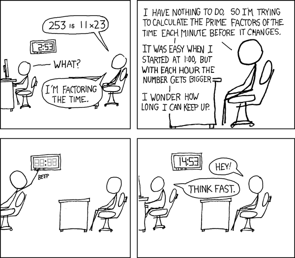
Figure 5.3.3.23. Factoring the Time.}{(`https://xkcd.com/247/`) I occasionally do this with mile markers on the highway.}
🔗

🔗

Prev Top Next